Simulations Atlas of Past Comets: 1700 to 1899

• C/1874 H1 Coggia

I had some hesitation deciding if the comet Coggia was mostly dust or mostly gas. The reason is that the spectroscopic observation mention both a continuum and gas, so both tails actually existed. However, only a single tail is mentioned, while gas tail and dust tail would have been separated. Thus, one of the tails must have remained below visibility threshold.

The fact that the spectral lines of C2 were visible is not decisive point, as even in rather dusty comets, they could show up as they are located very near the peak sensitivity of the eye in scotopic vision. Also, both the dust tail and the gas tail were straight and narrow, making it impossible only from the description to simply discard one or the other.

So, I simulated both cases, and found that dust tail gave a much better overall match of descriptions than gas tail. Thus, it means that the gas tail must have remained below visibility threshold despite the fact that gas was spectroscopically observed. The reasons dust tail gives a better match are:

• the length of tail reported, as only 6° at the beginning of July, growing to 45° mid-July, matches well with the simulations for a dust tail. For a gas tail, the length should have been longer in the beginning of July.
• The fact that the tail length kept growing to eventually 60° to 70° as the comet was approaching solar conjunction between 16^th and 23^rd of July also matches the dust tail.
• The fact that Trouvelot reports that, on evening of July 21^st, the tail reached the location of Gamma Ursa Majoris matches the expected location of the dust tail (beware, the Wikipedia page of comet Coggia mentions Gamma Ursa Minoris, while Trouvelot indeed mentions Gamma Ursa Majoris) while the gas tail was located in the southern hemisphere then.
• The fact that it is mentioned that comet Coggia last observation from the northern hemisphere was July 23^rd. at this date, the comet head had passed solar conjunction, and the dust tail was still located in the northern hemisphere, while the gas tail was located in the southern hemisphere
• Also, Comet Coggia drawings show the narrow “dark streak” behind the nucleus, typical of dusty comets (shadow of the dense nucleus area).

This choice has one drawback, that being mostly dusty, the comet should have exhibited a spectacular increase of brightness due to forward scattering, bringing it to magnitude -4.5 when in solar conjunction. So it could have been visible in daylight while no observations were reported. However it should be noted that comet Coggia was very near Earth, and must have been “relatively large”. Thus, like comet Tsuchinshan-ATLAS, it seems probable that it would not have been observed visually in daylight despite its actual brightness.

• C/1861 J1 Tebbutt

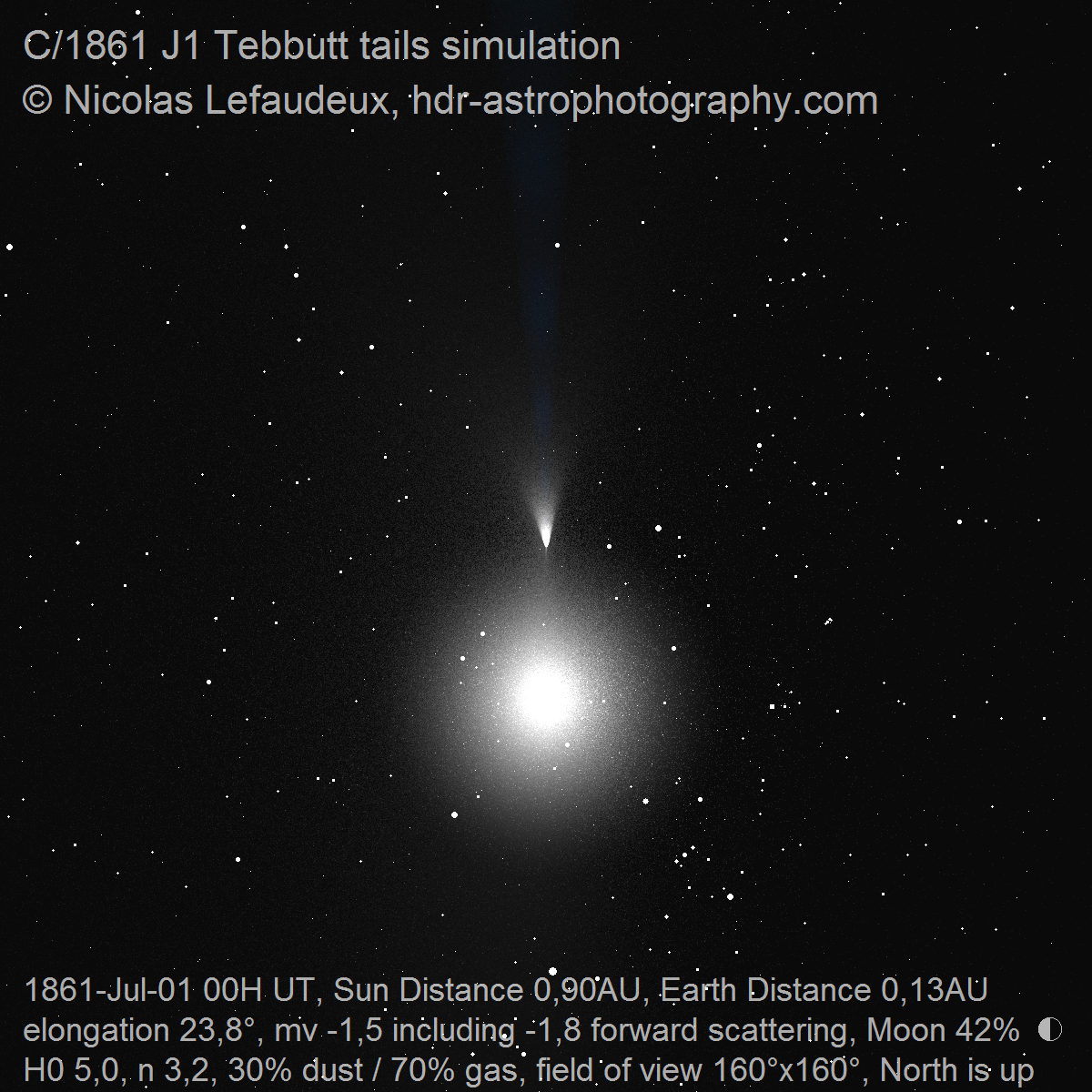
Comet Tebbutt appearance became one of the most spectacular comet thanks to the extraordinary encounter circumstances with Earth. Comet Tebbutt approach the Earth at only 0.13 AU, which is very rare, but the most extraordinary aspect was that, for a short time, Earth was indeed inside the dust tail of the comet.

The circumstances of the crossing of the tail of comet Tebbutt by Earth were virtually perfect. The Earth crossed the dust tail after perihelion, when it has been fully loaded by dust emitted around perihelion time. Also it seems from the simulations that the Earth went straight through the part of the dust tail made of the smallest dust particles, which is generally the densest part of the dust tail for most comets.

However, comparing the descriptions of the comet with the simulations, it seems that comet Tebbutt was indeed a very gaseous comet, with a not-so-rich dust tail. Descriptions of the comet before close approach to Earth mention a “main tail” that was long, and a shorter “secondary tail”. This description is matched only with a very gaseous comet, with the main tail being the gas tail, and the secondary tail the dust tail. Usually, most of the great comets are dusty, as the dust tail can be bright and spectacular, especially post-perihelion, while the gaseous tails are never bright. Thus for a gas tail to be qualified as a “main” tail requires the comet to be very gaseous.

Also, using a gaseous comet reduces the forward scattering brightness enhancement and is indeed compatible with the brightness reported. If comet Tebbutt had been more dusty, forward scattering enhancement would have been much stronger and comet Tebbutt would have probably been as bright as Venus at the time of close approach, while it was reported fainter than Jupiter. Eventually, reports of greenish hue of the comets are mentionned in the “Atlas of great comets” and the article “John Tebbutt and the great comet of 1861” relates the observation by Webb of a greenish hue on July 10th (golden hue reported on June 30th was probably from the combined effect of low elevation of the comet and forward scattering). It seems possible that comet Tebbutt was even more gaseous and with less dust than in the simulations.

The simulations show the development of comet Tebbutt in the southern sky as it approached Earth. Its size and brightness increased spectacularly from June 10^th to June 30^th. By June 20^th, it became a great comet. Yet, the full moon of June 22th must have interfered a lot with its visibility during the best time of the Earth approach between June 20^th and June 30^th.

On June 30^th morning, it began to be visible from the Northern hemisphere. According to http://www.phenomena.org.uk/comets/comets/comet1861.html: “the first person in England to see it may have been William C. Burder, of Clifton, Bristol, who dashed off a letter to the Times on Sunday, June 30th. “Sir – At 2.40 a.m. today I detected a brilliant comet near the north-west horizon. It was visible till 3.20 a.m….it appeared as bright as Capella and was favourably situated for the comparison. It was surrounded by a nebulous haze, but I saw no tail.”

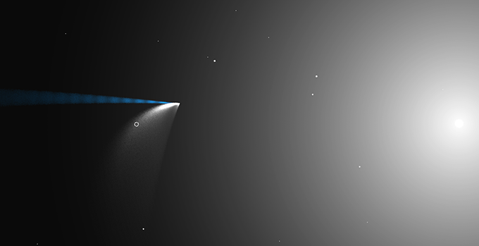
Indeed, the simulation show that at that time, the aspect of the comet must have been very unusual as the Earth was peering along the edge of the densest part of the dust tail, making it appear as a wide, mostly circular glow located on the side of the nucleus.

According to the simulations, the Earth entered the dust tail on June 30^th around 15h UT, went through the densest part around 21h UT, and exited around 3h UT on July 1^st. During the time, the appearance of the comet must have changed a lot. According to the simulation, the dust tail must have appeared a shifting triangular shape, that was initially rather short (shorter than 10°) and bent “to the right”, and progressively became longer (more than 30°) as it rotated counter clockwise “to the left”.

Looking at the famous drawing of comet Tebbutt by Williams at the time Earth was within the dust tail, the triangular head seems significantly larger and longer than in the simulations. It must be noted that, at the time the Earth was within the dust tail, the exact shape and length of the comet rendered by the simulation is very sensitive to the exact content and spread velocity of the dust particles. It is for sure possible to get a better match of the tail shape and length at that time by using a dust population marginally richer in smaller dust to get the tail longer, and faster spread velocity of the dust particles is larger to get a larger “angle” of the triangular head. Yet, as the match is already quite good with the standard comet model I used on all the comets simulations, those parameters have not been adjusted.

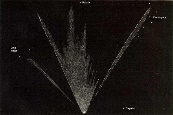
Besides the bright triangular head, the simulations shows a extremely large and diffuse glow filling a large part of the northern hemisphere sky at the time Earth was within the comet dust tail. Indeed, auroral glows have been reported at that time from various locations, and it seems realistic to consider those as being the dust tail of the comet. The simulation even renders some diffuse glow south of the sun, that might have been visible from the southern hemisphere reaching almost the antisolar direction.

animations with stretched intensities in the opposite direction of the sun and for southern hemisphere. The gas tail is seen rotating around the opposite direction of the sun, and a large glow is visible over most of the sky of the southern hemisphere at the time Earth was within the dust tail.

During the time of near approach to Earth, the gas tail is rendered reaching constellation of Aquila, about 120° from the comet head, which matches the very long tail lengths reported. Once the Earth exited the dust tail, the geometry became more usual and the dust tail quickly grew to reach about 60° in the first days of July before slowly shrinking as the comet got farther from Earth.

• C/1858 L1 Donati

Comet Donati is one of the most famous great comets. it was visible at large solar elongation, best placed for the northern hemisphere, in the evening, and for almost a full month. According to the simulations, the highlight of the display was between 1^st and 20^th of October 1858. During this period, the comet magnitude remained stable between magnitude 0 and -1, and the comet tail grew from less than 20° to more than 40° long while getting progressively less contrasted. At the end of the period, the moon light started to interfere with the view reducing the visible tail length.

• C/1843 D1, Great comet of 1843

The great comet of 1843 was one of the best Kreutz comet. it was seen in broad daylight, and displayed a long, straight and narrow tail when it got out of the sun glare. The simulation renders well the overall appearance of the straight and narrow tail, as well as the evolution of the length of the tail. The tail was around 20° when it emerged the sun glare on March 3^rd. it was then very narrow, and high surface brightness. Then the tail reached more than 40° on March 7^th, and remained about this length until March 23^rd while slowly fading. In the simulation, the maximum tail length is about 50° at the time of the full moon (March 16th).

• C/1811 F1 Flaugergues

Comet Flaugergues was quite similar to comet Hale-Bopp: a very large comet, with negative absolute magnitude, having a relatively remote perihelion, and quite not favorable geometric circumstances with always large distance from Earth. Yet, reports of comet Flaugergues suggest tail lengths relatively longer than comet Hale-Bopp. One reason is the slightly better circumstances for Flaugergues, with closest approach to Earth and largest elongation happening notably post-perihelion, while those were pre-perihelion for Hale-Bopp.

To simulate these longer tails, I also used a an absolute magnitude 0.5 magnitude brighter than Hale-Bopp and higher dust content. Despite this, the comet tail remains shorter in simulations than what was reported. This is one of the few notable discrepancy between simulation results and reality. In the simulation below, I artificially increased dust lifetime by about 25% to reach the observe tail length. I suspect one of the reason might be that comet Flaugergues was unusually rich in smaller dust particles. Indeed, on the only accurate drawing of the tails of comet Flaugergues with stars, the position of the tail in simulation is not at the actual drawing position. Getting the tail at the right position would require using smaller particles, which are spread more by radiation pressure and give longer tails.

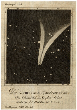
Comet Flaugergues drawing on September 10th evening and associated simulation. The position of the left branch of the tail matches the gas tail. The position and length of the right branch of the tail would match a dust tail with unsually small dust particles.

• C/1743 X1 Cheseaux

Comet Cheseaux is famous for having displayed a huge tail visible from northern hemisphere while the comet head was only visible from southern hemisphere. For this, it has been compared to comet McNaught. Yet, while comet McNaught was an average size comet significantly boosted by forward scattering, comet Cheseaux was a huge comet with absolute magnitude similar to Hale-Bopp. Even two weeks before perihelion, it was reported to be as bright as Venus. The simulation indeed renders the huge fanned tailed, with strong striation, but also show that the fanned tail must have been MUCH brighter than the one of comet McNaught. It seems that a fairer comparison would be to compare McNaught to a mini-Cheseaux comet!